SPRAT
Contents
- Introduction
- Current Status
- Specification
- Sensitivity
- Acquisition
- Data Reduction Pipeline
- Binning
- A note on flux calibration
- Filenames
- Multi-extention FITS data format
- Example data set
- Plotting with astropy, specutils and matplotlib
- Extraction using the Starlink software
- Extraction using DS9
- Wavelength Calibration
- Phase 1 Info
- Phase 2 Info
- RTML and Automated Spectral Followup
- Standards
Introduction
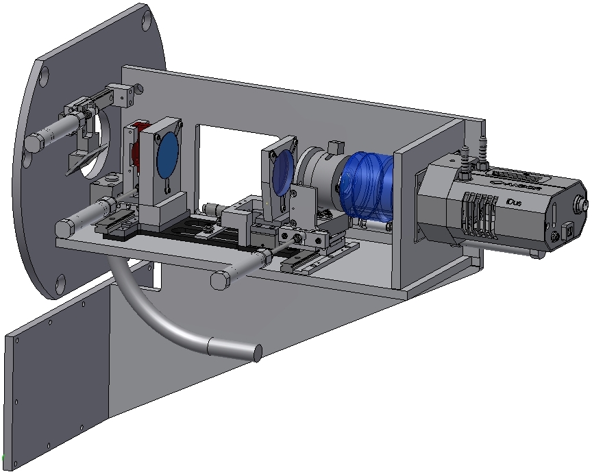
SPRAT (SPectrograph for the Rapid Acquisition of Transients) is a low resolution, high throughput spectrograph. It employs a VPH grating and prism ("grism") assembly to give a straight-optical path. The grism and slit are removed from the beam for acquisition and then placed in the beam for spectroscopy.
SPRAT was fitted to the telescope at the start of September 2014 and is in routine use, available to all observers. The adjustable slit is set fairly wide at 1.8 arcsec yielding a resolution of approximately R=350 (18Å).
Current Status
Specification
Camera
- Andor iDus 420 Series, 26.6 x 6.6 mm/1024 x 255 pixel CCD
- read noise: 2.34 ADU (5.7e)
- gain: 2.45
- approximate sensitivity for one photon per second per angstrom at 5500Å is V=16.5 [exposure time calculator]
- minimum exposure time=0.03s, limited by built-in shutter
- field of view in imaging (acquisition) mode 7.5 x 1.9 arcmin.
- spatial pixel scale 0.44 arcsec/pixel.
Grating
- Wasatch VPH model WP-600/600-25.4
- line density 600 lines/mm
- adjustable grating option — grating may be set to two different configurations optimized for "blue" or "red" throughput
- wavelength range 4020–8100Å
- order blocking filter cuts out all light below 4000Å
- dispersion 4.6Å/pixel (Slit limits the observed resolution.)
Slit
- width 1.8 arcseconds, giving a resolution of 18Å (4 pixels), corresponding to R=350 at the centre of the spectrum
- length 95 arcseconds
Lamps
- Xenon arc calibration lamp
- Tungsten flat field lamp
Sensitivity vs wavelength
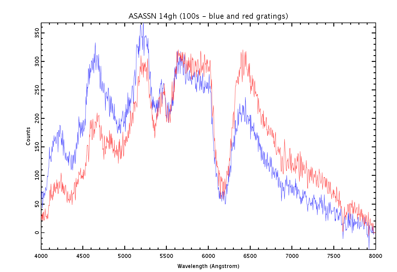
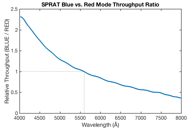
Our plan is to eventually provide absolute sensitivity curves for the two grating modes. In the meantime the example spectra below and the derived ratio plot show the difference in throughput between the two modes as a function of wavelength. The break-even point where the two modes offer equal efficiency is 5600Å. Switching between the modes takes < 10 seconds.
|
|
(Click on graphs to enlarge)
Acquisition
Acquisition with SPRAT uses the same concepts of "WCS FIT" or "BRIGHTEST" as implemented for FRODOspec . However, unlike FRODOSpec, acquisition imaging is done on the same detector as used for spectroscopy. This eliminates a source of error in changing instruments, and allows us to acquire onto the (relatively) narrow slit. This means you must have accurate coordinates (better than 1 arcsec) for your targets. Coordinate errors in large catalogues frequently exceed this, especially for moderate proper motion stars. We strongly recommend obtaining your own astrometry from a recent image wherever possible.
The acquisition process moves the target onto a "magic pixel" on the SPRAT CCD. The location of this pixel is maintained by operations staff and may vary slightly over time, though it should be close to 493,179 (updated 2023 Dec 04, subject to change). Targets should thus be located on or very close to this pixel in the final acquisition image obtained just before spectra are acquired. Note that all acquisition images are made available to users.
On a well-populated field the acquisition process usually takes 4-5 minutes. This includes time to take an image of the slit after acquisition, before the first spectral data are acquired.
Though relatively complicated, most users have no need to get involved in the acquisition process beyond providing accurate target coordinates. The "Wizard for SPRAT" option in the phase2ui automatically creates the optimum observing sequence.
NB: It is also possible to use IO:O to provide an acquisition image instead of SPRAT. In such a case the LT will adjust the telescope to place the target on the "magic pixel" in IO:O's field of view. Then it moves the science fold to select SPRAT and put the target on the slit. See "Using IO:O as the Acquisition Instrument" on the main SPRAT page for full details, and the implications of setting this up.
Data Reduction Pipeline
An adaptation of the FRODOSpec pipeline is being used to provide reduced, wavelength and flux calibrated 1d and 2d spectra for unbinned data. Both sky-subtracted and non-sky-subtracted versions are available. Access to the raw data is also provided. The intent of the automated pipeline is to provide science-ready data products for isolated, point source targets. Extended or crowded sources may be expected to require further input from the user.
Level 1 pipeline: All data pass through the "Level 1" pipeline to remove low level instrumental signatures. The same common-pipeline-software is used for all LT CCD and CMOS detectors. Corrections applied on SPRAT are a constant fixed-value bias, exposure dependent dark current and a flat field. Imaging and spectral data have their own separate flat fields because of the differing optics. Unique to SPRAT is a single-isolated-bad-pixel filter. Individual hot or cold pixels that exhibit extreme deviation from their neighbours are cleaned. Acquisition frames, slit images and arcs are treated as 2D images, reduced through the L1 pipeline and distributed as simple FITS image files like any other imager.
Level 2 pipeline: The spectral data are passed through a second "Level 2" pipeline to perform source detection, extraction, sky subtraction and wavelength and flux calibration.
Binning
We advise all users to only make unbinned observations for the time being. Although binning 2x2 is offered as an option on the Phase2UI, the binned data pipeline is still in development at time of writing.
A note on flux calibration
We make absolutely no claim that the automated pipeline provides precision spectrophotometry. The intention of the flux calibrated data products is exclusively to remove the instrument's own spectral response and provide a good representation of the true continuum colour. The pipeline makes no Telluric or airmass corrections and does not derive a nghtly atmospheric extinction profile. The instrumental spectral response used by the pipeline is only recalibrated following hardware changes or as required. It is not recalibrated frequently to trace the steady degradation of the mirror surface (LT Tech. Note 1: Telescope and IO:O Throughput) so can be expected to show significant drift (∼0.1 mag/yr) on long time-scales. Observers requiring the best spectrophotometry will need to schedule their own calibration standards.
Filenames
Filenames follow the usual LT conventions and are in the form "v_e_20170216_M_N_0_R.fits", where M and N uniquely identify the observation within the night and R is a status flag defining what level of processing has been applied.
| R | Description |
| 1 | Level 1 reduced image. This is the final product for arc, slit and acquistion images. The FITS contains a single primary array. |
| 2 | Level 2 reduced data products. This is a multi-extension FITS containing a primary image array that is the level 1 reduced CCD frame and up to five FITS extensions of derived products. If the pipeline was unable to successfully process the spectrum this *_2.fits file may not be created. |
| 0 | Raw data as read from the detector array. |
Multi-extention FITS data format
Level 2 data products (filenames ending _2.fits) are multi-extension FITS files containing a primary image array for the level 1 reduced CCD frame and up to five FITS extensions of derived products.
| Index | EXTNAME | Description | Example |
| 0 | L1_IMAGE | The "Level 1" reduced image. Basic CCD reductions have been applied but no spectral processing. | 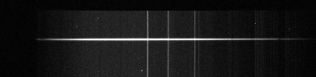 |
| 1 | LSS_NONSS | A wavelength calibrated long-slit image. No sky subtraction has been applied. A geometric distortion map has been applied to align the image array axes to spatial and spectral coordinates respectively. The wavelength axis has been resampled and linearized. This extension is most useful to observers of extended or binary targets since a wavelength calibrated spectrum of any point in the slit may be obtained simply as an indivdual pixel row. | 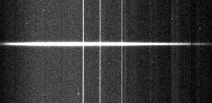 |
| 2 | SPEC_NONSS | Automated 1D extraction of the acquired target with wavelength calibration applied, but not sky subtraction. Extraction assumes a point source so may not be appropriate for extended, merged or crowded targets. This extension may not exist if the pipeline was unable to detect an isolated point source at the expected target location on the slit. | 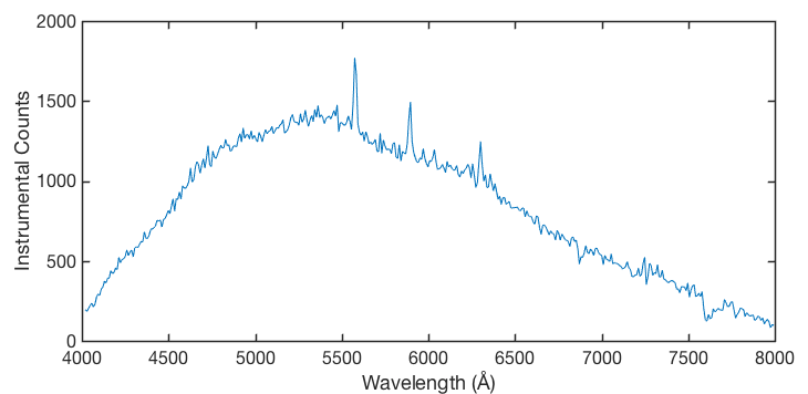 |
| 3 | SPEC_SS | Automated 1D extraction of the acquired target with wavelength calibration and automated sky subtraction applied. Sky subtraction assumes the darkest region of the slit is clean sky which may not be true for a target embedded in a larger nebulosity such as a supernova in a nearby host galaxy. See also description of SPEC_NONSS above. | 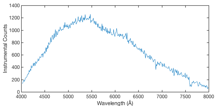 |
| 4 | NORMFLUX | Automated, wavelength calibrated, sky subtracted, 1D extraction, converted to normalised flux. That is, the instrumental spectral response has been removed to yield the target's correct relative flux as a function of wavelength. Units are normalised to average unity in the region 5000–6000Å. Always exists if extension SPEC_SS exists. | 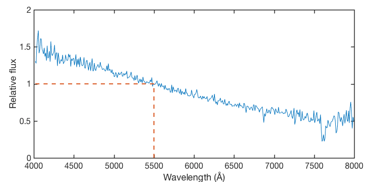 |
| 5 | FLUX | Automated, wavelength calibrated, sky subtracted, 1D extraction, flux calibrated in erg s-1 cm-2 Å-1. The absolute flux calibration is based on photometry of the final acquisition image, not of the spectrum itself. There are therefore no slit losses and approximately the same result would be extracted in very good or very poor seeing. This may have implications for extended sources where it is unclear how the aperture photometry has affected flux extraction in the image. May also be wrong in patchy cloud where extinction changes between acquisition and spectrum. This extension will not exist if the pipeline was unable to detect an isolated point source at the expected target location in the acquisition frame, if the image has unreliable photometry for any reason (e.g., saturated CCD) or if a native SPRAT acquisition image does not exist (e.g., acquisition was performed using IO:O). | 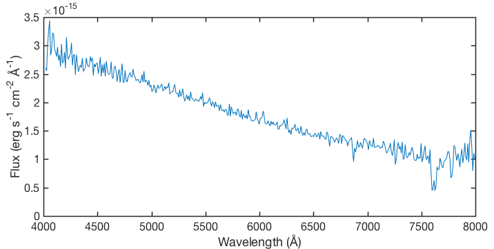 |
Example data set
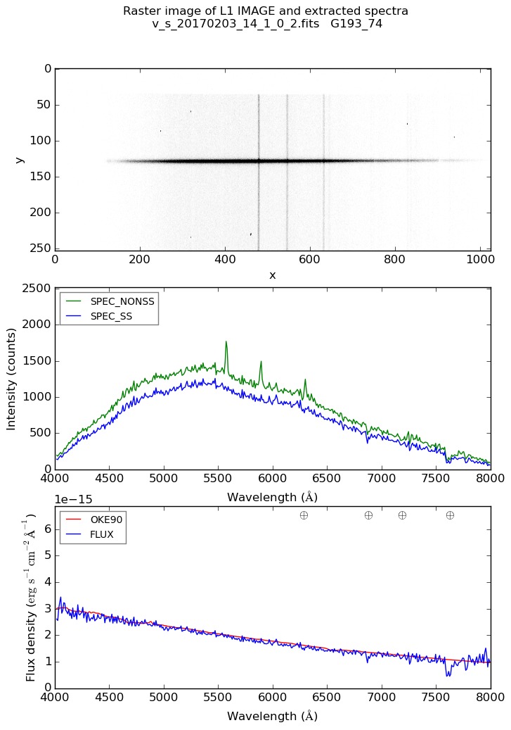
Shown is an example automated reduction for a 180sec integration of the V=15.7 standard star G193-74. Preview plots in this form are available for all observations from the LT data archive.
The top panel shows the basic CCD image before any spectral processing. This is the "Level 1" data product and found in the FITS primary image.
The centre panel shows FITS extensions 2 (SPEC_NONSS) and 3 (SPEC_SS), extractions of the target object presented in instrumental counts with and without sky subtraction. In the green SPEC_NONSS trace, sky emission lines are visible.
The bottom panel shows FITS extension 5 (FLUX), the final flux calibrated, wavelength calibrated spectrum in units of erg s-1 cm-2 Å-1. The pipeline provides no correction for Telluric absorption which is visible towards the red end of the spectrum. For comparison the data of Oke 1990 (AJ, 99, 1621, 1990) have been overplotted.
Plotting with astropy, specutils and matplotlib
Following is a minimal example of using specutils and Astropy to plot SPRAT spectra in Python.
    from astropy.io import fits
    from astropy import units as u
    from matplotlib import pyplot as plt
    from astropy.visualization import quantity_support
    import astropy.wcs as fitswcs
    import specutils as sp
    quantity_support()

    f=fits.open("FILENAME.FITS")

    # For SPRAT and LOTUS this is the Sky Subtracted Spectrum.
    # Other extensions are available!
    extension = 3

    # FITS are stored as 2D NAXIS1 x 1 arrays. Read and convert to a 1D NAXIS vector.
    specarray = f[extension].data
    specdata = specarray[0]
    specheader = f[extension].header
    f.close()

    flux = specdata * u.Unit("adu")

    # create WCS Wavelength Calibration, picking the required keywords from the fits header
    my_wcs = fitswcs.WCS(header={'CTYPE1':specheader['CTYPE1'], 'CUNIT1':'Angstrom',
                                 'CRVAL1':specheader['CRVAL1'], 'CDELT1':specheader['CDELT1'],
                                 'CRPIX1':specheader['CRPIX1'] })

    sp1d = sp.Spectrum(flux=flux,wcs=my_wcs) # create Spectrum objecti. Older versions of specutils may need sp.Spectrum1D()
    plt.plot(sp1d.spectral_axis,sp1d.flux)
    plt.show()
Also available for download is a small python script (sprat_splot.py) that uses the above method to plot any one of the SPRAT FITS extensions. It is only a minimal demonstration and not a full plotting application. Assuming you already have all the Python dependencies installed, it may be run:
    python sprat_splot.py v_e_20190905_7_1_0_2.fits -x 5
    python sprat_splot.py -h                                                # to get syntax help
If the pipeline selects the wrong target when several have landed in the slit or your target is extended and you want to isolate just a section of it, you can use the LSS extension as described above in 'Multi-extention FITS data format'. We provide a minimal demonstration script (sprat_splot_lss.py) of how to do that in Python, astropy and specutils. It may be run:
    python sprat_splot_lss.py v_s_20200809_99_1_0_2.fits 89 91              # Coadd three pixels rows from LSS_NONSS
    python sprat_splot_lss.py v_s_20200809_99_1_0_2.fits 89 91  -s 150 190  # Coadd three pixels with sky subtraction
    python sprat_splot_lss.py -h                                            # Command line help
Extraction using the Starlink software
Starlink users may extract the appropriate extension using the CONVERT:FITS2NDF command, appending the filename with the extension they wish to extract in brackets. The result is a single extension .SDF file. For example, to extract the wavelength calibrated, sky subtracted spectrum in units of instrumental counts, use:
  > convert
  > fits2ndf "v_e_20170116_1_1_0_2.fits[3]" wcscomp=axis
  > fits2ndf v_e_20170116_1_1_0_2.fits\[3\] wcscomp=axis
Or alternatively, you can access the required HDU by using the corresponding EXTNAME key:
  > fits2ndf "v_e_20170116_1_1_0_2.fits[SPEC_SS]" wcscomp=axis
  > fits2ndf v_e_20170116_1_1_0_2.fits\[SPEC_SS\] wcscomp=axis
Extraction using DS9
DS9 users may view a mosiac of all available extensions using the -multiframe command line option or else specify the extention by number:
  > ds9 -multiframe v_e_20170116_1_1_0_2.fits
  > ds9 v_e_20170116_1_1_0_2.fits\[1\]
  > ds9 "v_e_20170116_1_1_0_2.fits[1]"
A frame extraction can be achieved with the -savefits parameter.
> ds9 v_e_20170116_1_1_0_2.fits\[1\] -savefits output.fits -quit

Wavelength Calibration
We recommend that all users include a Xenon arc observation at the end of their group (see the SPRAT Phase2 guidelines for details). This arc will be used by the pipeline to wavelength calibrate spectra extracted from your data. If you do not include an arc in your observing sequence the pipeline will automatically use the best matching arc available to it from the data archive.
This (below) is a simple arc map showing normalised Xenon arc line strengths in both the red and blue-optimised grating modes, annotated with selected lines..
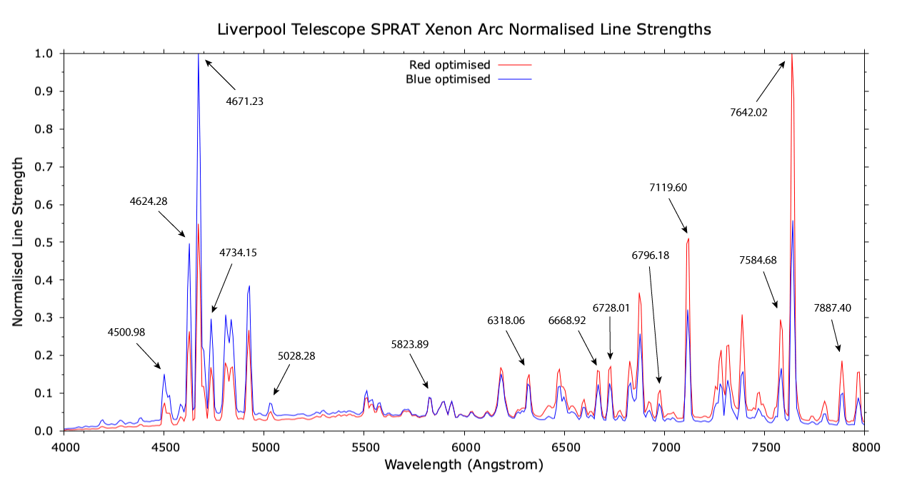
click for bigger version |
Text files used to produce these arc line curves -
|
Phase 1 Info
SPRAT is available for common user applications from Semester 2015A onwards. You should be aware of the following overheads:
- Acquisition Time (slew plus accurate acquisition): 4 minutes
- Readout Time: 10 seconds
- Grating Mode (blue/red) change: 10 seconds
- Xenon Arc Exposure (recommended at start or end of exposure): 10 seconds
- [Tungsten Lamp Exposure (not routinely obtained or usually required): 10 seconds ]
Phase 2 Info
Guidelines on how to prepare observations are given in the Phase 2 web pages. Note in particular the instrument-specific User Interface Instructions. The phase 2 "Wizard" should always be used to prepare observations. Groups that can not be prepared with the wizard should be discussed with LT Phase 2 support. Note that LT staff do not routinely check observing groups, and that observing groups are potentially active as soon as they are submitted. Please do contact us if you have any questions about your observations.
RTML and Automated Spectral Followup
SPRAT can accept observation requests formatted in Remote Telescope Markup Language (RTML), which allows you to automatically trigger certain observations from within your own autonomous software. We provide a command-line-based utility which can format RTML packets for you, making it easy to integrate observing requests into a shell script or other data processing pipeline. For some user cases it might also be easier for users to upload all their observing requests from the command line instead of using the Phase2UI. The RTML facility is available to all users who have TAG-awarded time allocations. Please contact us if this sounds of interest, and we will provide full user instructions.
Standards
A single spectrophotometric standard observation is performed on any nights that are anticipated to offer photometric clarity. This provides routine monitoring of overall system throughput and stability and the exposures are available to all observers. A single standard observation is not sufficient for precision spectrophotometry and will not, for example, allow derivation of a night-specific atmospheric absorption. Users requiring a higher level of photometric or atmospheric calibration must schedule their required standards from their own time allocation.
Users may wish to add a standard star observation to their SPRAT observing sequence so that their calibration observations are matched in time and airmass with the science data; see the SPRAT Phase2 guidelines for details on how to do this using the Sequence Builder. Links to tables of spectro-photometric standard stars are provided by ESO here, however it should be noted that very many of the common spectro-photometric standards are high proper motion stars and published catalogue coordinates are inadequate for slit acquisition. A selection of popular standards for which we maintain up to date coordinates is preconfigured in the phase2ui when you select "Add Target" in the phase2ui.
When choosing which standards to use, Marco Lam's Spectroscopic Standards Web Viewer (DOI 10.5281/zenodo.7978970) is very helpful.